On 8 September 2026 Britain's electricity grid had an expensive day. By our count the grid operator paid £33.6 million in 24 hours to generators to change what they were doing, to keep the system in balance. When we looked at the wind data for the day, something stood out. The forecast had predicted nearly 17 gigawatts of wind generation, on average, across the day. The wind farms produced far less. At first glance it looked like a spectacular forecasting error, roughly 5 gigawatts, in every hour of the day. Was the forecast really that bad? And if it was not, why was the day so expensive? This article follows the public data step by step, for readers new to energy trading and weather forecasting.
Jordan Dimov (A115) and Gökberk Görür (quantitative meteorologist). Published 10 October 2026. Sources and technical notes are at the end.
1. An expensive day on Britain's grid
Electricity must be balanced continuously. Supply has to match demand second by second, and the power has to be able to get from where it is generated to where it is used. Storage helps, but it cannot remove every mismatch or every bottleneck in the wires. In Great Britain the National Energy System Operator (NESO) does the balancing. When the market leaves the system short or long, or when a transmission route cannot carry all the power behind it, NESO pays generators to change what they are doing. The marketplace for those instructions is the balancing mechanism.
A word on the £33.6 million, because there is more than one way to count a day like this. Ours is the simplest: add up everything NESO paid generators for those instructions, using the cashflows Elexon publishes for each one. Some money flows the other way too, and netting it off leaves £31.6 million. Other trackers try to isolate the extra cost of the network bottlenecks alone, and they put this day at around £30 million. The definitions differ, the size does not. Whichever way it is counted, the money is recovered from electricity consumers through network charges. The technical notes at the end give the exact definition.
2. The strange wind forecast
NESO publishes a wind generation forecast called WINDFOR. It is hourly and it is re-issued eight times a day. We took the last issue published on the afternoon of 7 September, at 16:30, which is the last complete view of the next day before delivery began, and lined it up against the metered output of the wind farms hour by hour. Figure 1 shows the result.
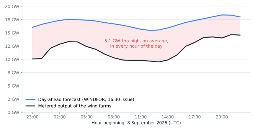
The forecast averaged 16.9 GW across the day. The farms produced 11.8 GW. The gap was 5.1 GW, and the forecast was above the outturn in all 24 hours. It was never once too low.
When we first plotted this, the forecast looked terrible. But something about the picture was odd. The gap barely moved as the wind rose and fell through the day. A forecast that is wrong by the same amount, in the same direction, all day long is usually a sign that the comparison is wrong, not the forecast. So we went to look at what the grid operator had told the wind farms to do.
3. What the chart does not show
In the balancing mechanism, a generator can offer to reduce its output at a price. That offer is called a bid. When NESO accepts a bid, the generator turns down and is paid at the bid price. The accepted volumes are published after the day, unit by unit and half hour by half hour.
On 8 September NESO accepted wind bids in every one of the day's 48 half-hour settlement periods. This is where the money went: £3.8 million to wind farms paid to reduce generation, across 77 wind units, and £26.8 million to gas plants paid to increase generation, at an average of £230 per megawatt hour against a market price of £147 over the same periods. So the metered line in Figure 1 is not what the wind would have let the farms produce. It is what they produced after being told to produce less. To judge the forecast you have to put the withheld output back. For each of the 232 wind units that settle in the balancing mechanism, we added the accepted bid volume to the metered output. Figure 2 shows the result.
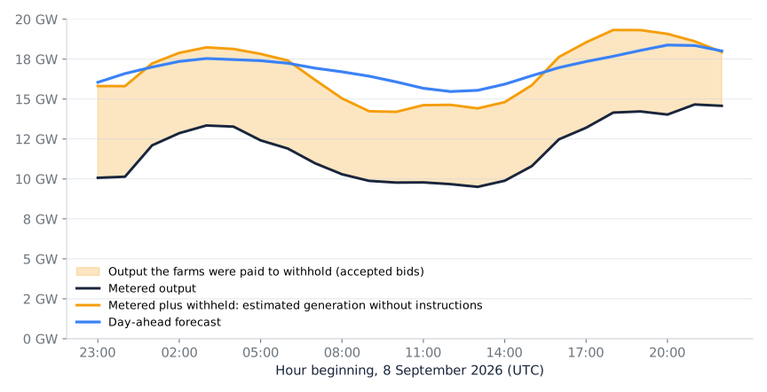
Most of the gap disappears. The accepted wind reductions averaged 4.95 GW across the day, and the gap between forecast and metered output matched them to within three per cent. Against the estimated generation without balancing instructions, the forecast's mean absolute error over the 24 hours was 0.86 GW, about five per cent of the day's wind, and its average signed error was +0.16 GW. The forecast ran a little high in the morning, when the wind fell further than expected, and a little low in the evening, when it recovered more than expected.
Two cautions belong here. The first is that the rebuilt series is an estimate, not a measurement. Accepted bid volumes are defined against the output each farm said it intended to produce, and intentions are not the same as physical capability. We call the series "estimated generation without balancing instructions" for that reason. The second is that the residual depends on which wind farms you count. Measured against the transmission system's five-minute wind total instead of the 232 units, the forecast comes out about 1.1 GW too low rather than 0.16 GW too high. The populations differ, and so does the answer. What does not change is the main point: the 5 GW was curtailment, not forecast error. Others reading the public data reached the same conclusion on the day itself; Kilowatts published a note that evening saying the gap "has essentially nothing to do with forecasting". The technical notes at the end set out the populations and the reconciliation.
Two kinds of error
The signed error is forecast minus actual, averaged with its sign, and it tells you whether a forecast leans high or low. The absolute error drops the sign before averaging, and it tells you how far off a typical hour was. Both matter, because a forecast that is too high half the day and too low the other half can have a signed error near zero and still miss by a lot in any given hour. That is this forecast: +0.16 GW signed, 0.86 GW absolute.
4. Why would Britain pay wind farms to stop?
An outsider's first question is usually this one. If a wind farm produces electricity it sells it and gets paid. If it stops, surely it just earns nothing. Why would anyone pay it to stop?
The answer is that by the time the operator needs it to stop, the farm has usually already sold the power. It sold it the day before, or earlier, to a supplier or a trader, and it may also earn a subsidy per unit generated. Turning down changes its commercial position: it still has to deliver what it sold, so it has to buy that power back in the market, and it loses the subsidy. The balancing mechanism lets each generator put a price on changing its output. Some wind farms would pay to turn down, some need to be paid, and the amount depends on each one's contracts and its bid. On 8 September, the wind farms that turned down were paid, and NESO then bought replacement power from generators in places the network could reach.
That is the second half of the answer: location. Britain's wind is mostly in Scotland and the North Sea. Much of its demand is in the south. The transmission routes between them can carry only so much, and on a windy day with low demand they fill up. Having enough electricity in total is not the same as being able to deliver it where it is needed. The first is an energy balance problem. The second is a network constraint. Most of the money on 8 September went on the second.
That also answers a natural follow-up: if demand was low, why was so much paid to gas plants? Low demand does not mean no demand. The south still needed power, and the market had already arranged to meet part of it with the northern wind that was now being turned down. Every megawatt hour withheld behind the bottleneck had to be replaced by one from a generator the network could reach, and south of the bottleneck that mostly means gas plants, paid at their offer prices. The wind reductions were the cheap half of a pair of instructions. The replacement was the expensive half.
| What happened on 8 September | Amount |
|---|---|
| Wind output withheld on instruction, average across the day | 4.95 GW |
| Energy withheld over the day | 119 GWh |
| Paid to wind farms to reduce | £3.8m |
| Paid to gas plants to increase | £26.8m |
| Average price paid to gas, against a market price of £147 | £230 per MWh |
| Total paid out on balancing instructions | £33.6m |
Table 1. The money and the energy. Not every gas instruction that day was a direct replacement for a wind instruction, and we have not classified each one, so the two rows are not a one-for-one pair.
Prices and incentives matter here, and they are the part of the story a trader should watch. Each wind farm tells NESO, before each half hour, what it intends to produce. These declarations, called physical notifications, set the baseline against which a reduction is measured and paid. On 8 September the declarations of the 227 units that submitted them averaged 17.9 GW, about 1.1 GW above our estimate of what the same units could have generated. One day's aggregate cannot say which farms, or why. But the pattern is not new: in 2024 Bloomberg reported that a large share of British wind farms had been overstating expected output, and the regulator opened an investigation. Separately, in May 2024 one offshore wind farm paid £33 million in redress after admitting it had submitted excessive bid prices during transmission constraints. Those are different issues from a bad forecast, and nothing here is evidence of either on this day. They are a reminder that the balancing bill is set by prices and declarations as well as by the weather.
5. Was the weather forecast actually wrong?
Adding back the curtailment still leaves an error of just under a gigawatt in a typical hour. Where did it come from? Forecasting wind power involves two questions: how windy will it be, and how much electricity will the turbines make in that wind? The first is a weather forecasting problem. The second depends on the turbines, their locations, their sizes and how many are available. Figure 3 shows why the second step matters: below rated wind speed a small error in wind speed makes a large difference to output, because output rises with the cube of the speed.
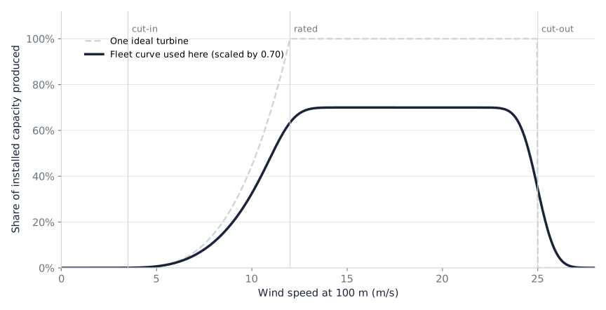
To separate the two, we built our own estimate of the day's wind power from scratch. We took the European weather centre's ensemble forecast issued the morning before, a reanalysis of the weather that actually happened, the positions of 6,129 turbines, and a published power curve fitted to seven and a half years of history with 8 September left out. Running the forecast weather and the actual weather through the same conversion tells you how much of the error came from the wind field itself.
The answer is about a quarter of a gigawatt. The forecast wind was slightly too strong, by 0.25 to 0.30 GW of power, and that result held whichever way we calibrated the conversion. Our independent estimate of the day's wind also agreed with the rebuilt series from the balancing data to within the model's own uncertainty, which is a useful check from a different direction. Beyond that, the split is not reliable. We tried three reasonable ways of calibrating the conversion. All three reproduced the overall forecast error, but they disagreed about how much of it came from turning wind into megawatts and how much from the differences between our method and NESO's. The forecast ensemble's own members also disagreed with each other by more than the quantities we were trying to separate. So we report the weather term and stop there.
Two limits should be said plainly. The weather result is a result for one ECMWF run and one reanalysis, not a measurement of NESO's whole forecasting system, which blends two weather models and its own corrections. And one day cannot say whether this forecast was better or worse than usual. What it can say is that the enormous error the first chart appeared to show was not there.
6. What could have reduced the bill?
We have not simulated what a different forecast would have done to the day's trading, scheduling and balancing actions, so we cannot put a number on what better forecasting would have saved. What the evidence supports is narrower. The operator knew, the day before, how much wind was coming, to within a gigawatt or so on a 17 GW day. It also knew where. NESO forecasts wind farm by farm, so it could see that most of the power would be in the north and that the routes south would be full. Knowing that does not create wire capacity. Britain's wholesale market trades the whole country at a single price, so the day-ahead market sold the Scottish wind to southern demand as if the wires did not exist, and the operator then had to undo that in the balancing mechanism, however clearly it had seen the day coming. The expensive part was not the forecast. It was the gap between where the market put the power and where the network could carry it, and the £230 per megawatt hour it cost to close that gap.
Forecasting, network capacity and market design address different problems. A better forecast helps the operator plan reserves and the market trade closer to reality. It does not add capacity to a transmission route. More wires do, but take years and cost billions. Making better use of existing wires through monitoring and operating practice can be faster. Storage and flexible demand help where they sit in the right place. Changes to how constraints are priced and who pays alter the incentives of everyone who bids. None of these is free, and none alone removes a day like 8 September. The useful question is which of them lowers the total cost most once its own cost is counted, and that is a different investigation.
7. The lesson
The apparent forecasting failure was misleading. Once we accounted for the electricity the wind farms were instructed to withhold, the 5 GW gap was gone, and an independent weather analysis found no sign of the error the first chart appeared to show. It could not reliably split the remaining gigawatt, and we say so.
None of this proves that better forecasting has no value. But on this day the harder problem was not predicting how much electricity Britain could generate. It was getting that electricity to where it was needed, at a price set by the generators the operator could reach. That problem involves wires, operating decisions and the incentives written into the market.
For a newcomer the durable lesson is about reading numbers. Public market data can lead a plausible analysis to a wrong conclusion in one step. Before you compare two series, ask who is in each. Before you call a gap an error, ask whether someone was instructed to create it. And before you read meaning into a residual, ask how large the uncertainty is on each side of the subtraction.
Technical notes
Data. Forecasts are NESO's WINDFOR as published through Elexon Insights, all 16 issues of 7 and 8 September 2026; the article uses the 16:30 issue of 7 September. It is the last issue before delivery, not an issue available before the day-ahead auctions, which close in the morning; a test of what a day-ahead trader could have known would use the 08:30 issue. Metered output is Elexon B1610 for the 232 wind balancing units. Accepted reductions are Elexon DISPTAV tagged bid volumes for the same units; the tagged type is the one that reconciles with the day's settlement totals. The reductions were cross-checked against the individual balancing instructions (BOALF), integrating each instruction against the unit's declared plan, and the two totals agreed to within 0.2 per cent. Cost figures are Elexon's indicative balancing cashflows (EBOCF) for the settlement day, positive rows summed. Settlement day 8 September runs from 23:00 UTC on 7 September.
Populations. WINDFOR covers wind farms visible to the operator with operational metering. The five-minute fuel mix (FUELINST) covers transmission-connected wind. B1610 covers the 232 wind balancing units. These are three overlapping but different sets, and smaller farms on local networks are in none of them. Against B1610 plus accepted bids (same 232 units on both sides) the day-ahead forecast error is 0.86 GW absolute and +0.16 GW signed. Against FUELINST plus the same accepted bids, the metered mean is 13.1 GW, the rebuilt series averages 18.1 GW and the forecast error is 1.4 GW absolute and minus 1.1 GW signed. The Kilowatts note of 8 September quotes 17.0 GW forecast and 13.3 GW metered, which matches the FUELINST basis. We prefer the B1610 basis because the bid volumes belong to the same units, but neither is proven to match WINDFOR's population exactly. The fact that the forecast-to-metered gap equals the accepted bid volume to within three per cent on the B1610 basis suggests the match is close.
The hourly comparison. All figures in gigawatts, hourly means, B1610 basis.
| Hour (UTC) | Forecast | Metered | Withheld | Est. without instructions | Error |
|---|---|---|---|---|---|
| 23:00 | 16.0 | 10.1 | 5.7 | 15.8 | +0.2 |
| 00:00 | 16.6 | 10.1 | 5.7 | 15.8 | +0.8 |
| 01:00 | 17.0 | 12.1 | 5.1 | 17.2 | -0.2 |
| 02:00 | 17.4 | 12.9 | 5.0 | 17.9 | -0.5 |
| 03:00 | 17.5 | 13.3 | 4.9 | 18.2 | -0.7 |
| 04:00 | 17.5 | 13.3 | 4.9 | 18.1 | -0.7 |
| 05:00 | 17.4 | 12.4 | 5.4 | 17.8 | -0.4 |
| 06:00 | 17.2 | 11.9 | 5.5 | 17.4 | -0.2 |
| 07:00 | 16.9 | 11.0 | 5.2 | 16.2 | +0.7 |
| 08:00 | 16.7 | 10.3 | 4.7 | 15.0 | +1.7 |
| 09:00 | 16.4 | 9.9 | 4.4 | 14.2 | +2.2 |
| 10:00 | 16.1 | 9.8 | 4.4 | 14.2 | +1.9 |
| 11:00 | 15.7 | 9.8 | 4.8 | 14.6 | +1.1 |
| 12:00 | 15.5 | 9.7 | 5.0 | 14.6 | +0.8 |
| 13:00 | 15.5 | 9.5 | 4.9 | 14.4 | +1.1 |
| 14:00 | 15.9 | 9.9 | 4.9 | 14.8 | +1.1 |
| 15:00 | 16.5 | 10.8 | 5.1 | 15.9 | +0.6 |
| 16:00 | 17.0 | 12.5 | 5.2 | 17.6 | -0.7 |
| 17:00 | 17.3 | 13.2 | 5.3 | 18.6 | -1.2 |
| 18:00 | 17.7 | 14.2 | 5.2 | 19.3 | -1.6 |
| 19:00 | 18.0 | 14.2 | 5.1 | 19.3 | -1.3 |
| 20:00 | 18.4 | 14.0 | 5.0 | 19.1 | -0.7 |
| 21:00 | 18.4 | 14.7 | 4.0 | 18.6 | -0.3 |
| 22:00 | 18.0 | 14.6 | 3.4 | 17.9 | +0.1 |
| Day | 16.9 | 11.8 | 5.0 | 16.8 | 0.86 abs., +0.16 signed |
The weather test. Forecast weather is the ECMWF IFS ensemble, 00Z run of 7 September 2026, 50 perturbed members, 100 m wind at three-hourly steps, so the test covers eight points of the day. Reference weather is ERA5 100 m wind, February 2019 to 7 September 2026. Turbine positions are from OpenStreetMap (6,129 turbines, 155 physical farms, 229 of 233 units and 99.6 per cent of capacity located; four supplier aggregates excluded). Wind is sampled at each turbine and averaged over the farm; farms are weighted by the registered capacity of their units, counting only units that had started reporting by that hour, so the fleet grows from 16 GW in 2019 to 30 GW in 2026. The conversion is a smoothed fleet power curve of the kind described by Olauson (2018) and Staffell and Pfenninger (2016): cubic from 3.5 to 12 m/s, flat to 25 m/s, Gaussian-smoothed with a 1.5 m/s standard deviation, with two fitted parameters, a wind speed scale and an availability scale. Fitted by least squares on three windows with 8 September excluded: the full period, the last twelve months, and August 2026. The fitted parameters were 1.005 to 1.025 for wind speed and 0.70 to 0.735 for availability; in-sample hourly RMSE was 0.93 to 1.18 GW, 12 to 13.5 per cent of mean output.
With the conversion frozen, the signed forecast error splits into three additive terms: weather (forecast weather through the curve minus reference weather through the curve), conversion (reference weather through the curve minus the rebuilt series), and the difference from NESO's published forecast (NESO's forecast minus forecast weather through our curve). The third term is not an isolated measure of NESO's method: it also carries our model choices, our reference weather, the mismatch between a 00Z weather run and a 16:30 forecast issue, and any population difference.
| Signed mean over eight hours (GW) | Full window | Last twelve months | August 2026 |
|---|---|---|---|
| Weather | +0.25 | +0.25 | +0.30 |
| Conversion | +1.06 | +0.11 | -0.06 |
| Difference from NESO's published forecast | -1.10 | -0.16 | -0.04 |
| Forecast error (the sum) | +0.20 | +0.20 | +0.20 |
| Ensemble spread (member standard deviation, hourly) | 1.45 | 1.40 | 1.45 |
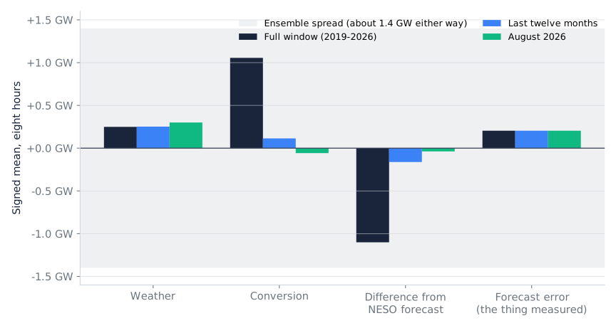
The tests that would count as failure were written before the run. Two fired: the conversion term changed sign across calibration windows, and the ensemble spread exceeded every term. The first is the decisive one. The spread is the standard deviation of the 50 members' hourly power, which is not the same thing as the uncertainty of an eight-hour mean, and members can share biases that the spread does not show; it is reported as context, not as a detection threshold. The in-sample RMSE is likewise context for the model's scatter, not an out-of-sample validation. The weather term's stability across windows is the result we rely on, and it is a result for this ECMWF run and this reanalysis.
References.
- Hersbach, H. et al. (2020). The ERA5 global reanalysis. Quarterly Journal of the Royal Meteorological Society, 146(730), 1999-2049.
- Olauson, J. (2018). ERA5: The new champion of wind power modelling? Renewable Energy, 126, 322-331.
- Staffell, I. and Pfenninger, S. (2016). Using bias-corrected reanalysis to simulate current and future wind power output. Energy, 114, 1224-1239.
- National Energy System Operator (2026). Energy Forecasting Strategy and Delivery Plan: the future of energy forecasting to 2030 and beyond.
- Kilowatts (8 September 2026). Britain just set a curtailment record, and the forecast was never wrong. dispatches.kilowatts.io.
- Bloomberg (2 February 2024). UK minister condemns energy firms for overstating wind farm output.
- Ofgem (28 May 2024). Beatrice Offshore Windfarm Ltd to pay £33.14m into the redress fund over excessive bid prices under the Transmission Constraint Licence Condition.